Consistent Signals
Table of Contents
One way in which a brand is supposed to be able to create greater brand recognition is through consistent use of signals, e.g., taglines, slogans, characters, and colors. But assessing consistency in a more than anecdotal way can be difficult, particularly if you don’t have direct access to the creative.
This is an attempt at assessing consistency via the open source resource, MOAT. We’re going to scrape the images from MOAT, read in the images and use the image_quantize() function from the magick package to extract the top 5 colors, and then look for a useful way of visualizing the data.
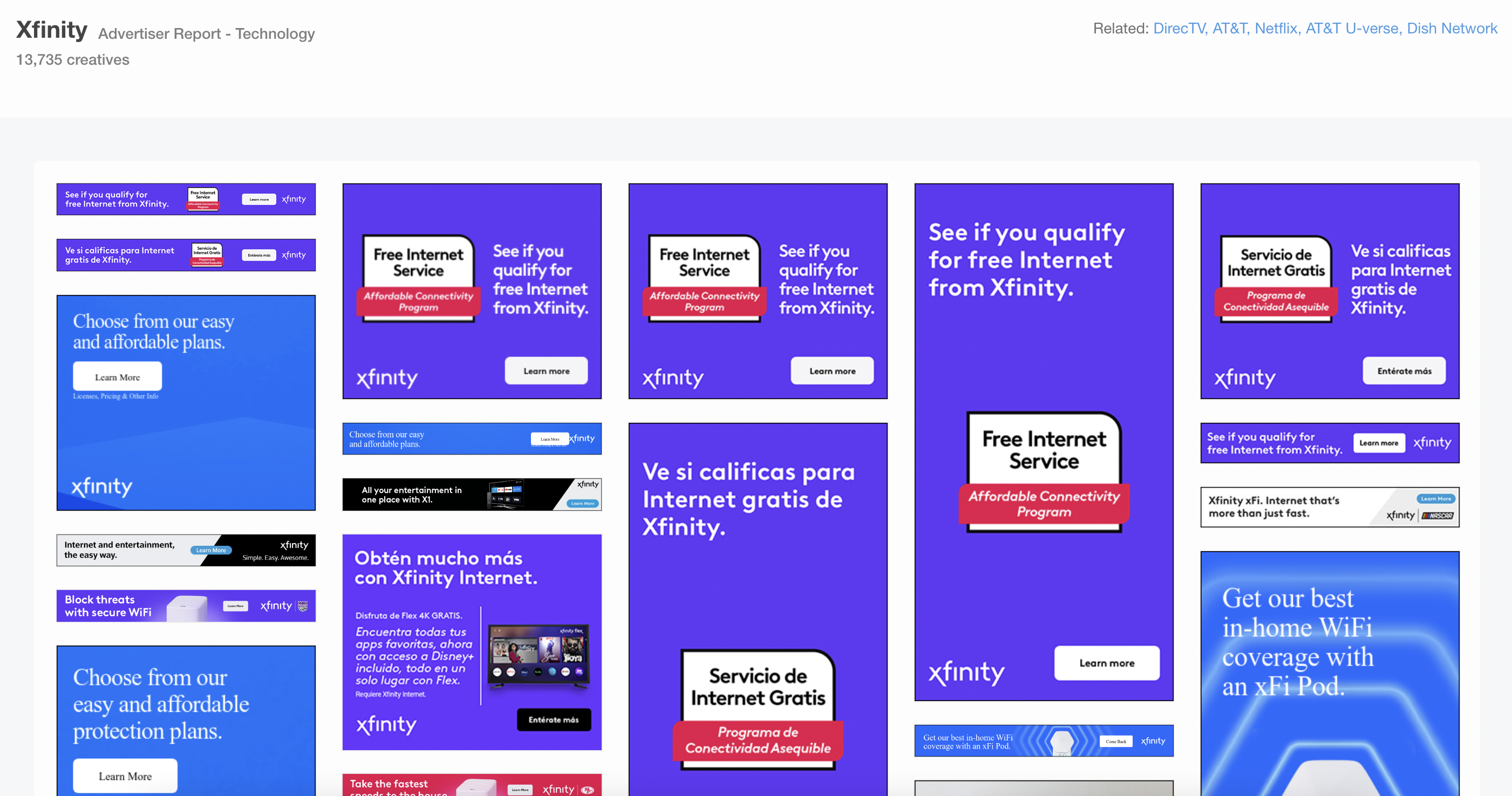
Figure 1: MOAT keeps a running collection of most brands display advertising
Getting the data
The first thing we have to do is actually get the data from the MOAT site. But when we go to inspect the site for scraping we find that the site is dynamically loaded using javascript, so we can’t simply scrape the image urls via rvest. But as pointed out in this post, this isn’t as big a deal as it seems -
Contrary to popular belief, you do not need any special tools to scrape websites that load their content via Javascript. In order for the information to get from their server and show up on a page in your browser, that information had to have been returned in an HTTP response somewhere.
To see that HTTP response, we can simply move over to the Network tab in our Chrome DevTools and reload the site to see which requests are being sent. In the image below, we can see the requests made on load. By clicking into each one we can see the response and if data is coming back. Scrolling through the response of the request highlighted in blue, we can see that this is the GET request that we’re interest in.
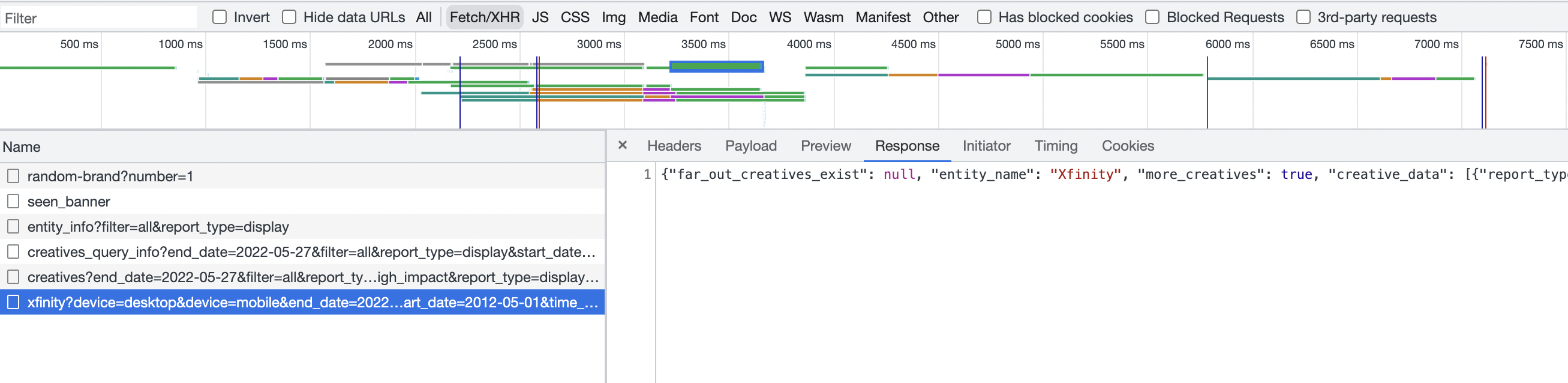
Figure 2: Requests made on load (left) and the response (right)
The next step is to build a GET request that matches what MOAT is using so that the same data will be sent to us. Luckily, the curlconverter makes it simple for us to do this. We just have to right-click the highlighted GET request and “copy as cURL”. The site will then provide us the cookies, headers, parameters, and the formatted GET request to send to the site servers.
library(httr)

cookies = c(
  's_fid' = '0D24F1992ADB7B2F-1A43B04BDAF89740',
  's_nr' = '1653840871687-New',
  'gpw_e24' = 'no%20value',
  's_cc' = 'true'
)

headers = c(
  `Accept` = '*/*',
  `Accept-Language` = 'en-US,en;q=0.9',
  `Connection` = 'keep-alive',
  `Content-type` = 'application/x-www-form-urlencoded',
  `DNT` = '1',
  `Referer` = 'https://moat.com/advertiser/xfinity',
  `Sec-Fetch-Dest` = 'empty',
  `Sec-Fetch-Mode` = 'cors',
  `Sec-Fetch-Site` = 'same-origin',
  `User-Agent` = 'Mozilla/5.0 (Macintosh; Intel Mac OS X 10_15_7) AppleWebKit/537.36 (KHTML, like Gecko) Chrome/102.0.5005.61 Safari/537.36',
  `cache-control` = 'no-cache',
  `pragma` = 'no-cache',
  `sec-ch-ua` = '" Not A;Brand";v="99", "Chromium";v="102", "Google Chrome";v="102"',
  `sec-ch-ua-mobile` = '?0',
  `sec-ch-ua-platform` = '"macOS"'
)

params = list(
  `device` = c('desktop', 'mobile'),
  `end_date` = '2022-05-27',
  `filter` = 'all',
  `load_time` = '1653840872',
  `page` = '0',
  `page_size` = '42',
  `period` = 'month',
  `report_type` = 'display',
  `start_date` = '2012-05-01',
  `time_hash` = '7239614689297618916'
)

res <- httr::GET(url = 'https://moat.com/creatives/advertiser/xfinity', httr::add_headers(.headers=headers), query = params, httr::set_cookies(.cookies = cookies))
Our cookies should remain consistent, so those can just be loaded once. Within the headers object we can see the base url and the path containing the brand we’re searching for. For this use case, the params object is the one of interest. We can see that we our GET request started on page “0” and that it returned data on 42 pieces of creative. Since we’re only going to focus on one brand at a time, we’re going to write a function that will iterate over a series of pages, and extract data from the 42 assets on each page. Additionally, if we run this code as is it will return an error. This is because there are two devices in our params, if we delete “mobile” and keep only desktop, it will work.
After running a single GET request and seeing how our data is structured and the variable names we’re interested in, we can write a function that will iterate over multiple pages and extract the relevant data into a data frame.
library(httr)
cookies = c(
  's_fid' = '004F9EEAE39BB8B2-268DC9087E86114D',
  's_nr' = '1653841705341-New',
  'gpw_e24' = 'no%20value',
  's_cc' = 'true'
)

headers = c(
  `Accept` = '*/*',
  `Accept-Language` = 'en-US,en;q=0.9',
  `Connection` = 'keep-alive',
  `Content-type` = 'application/x-www-form-urlencoded',
  `DNT` = '1',
  `Referer` = 'https://moat.com/advertiser/xfinity',
  `Sec-Fetch-Dest` = 'empty',
  `Sec-Fetch-Mode` = 'cors',
  `Sec-Fetch-Site` = 'same-origin',
  `User-Agent` = 'Mozilla/5.0 (Macintosh; Intel Mac OS X 10_15_7) AppleWebKit/537.36 (KHTML, like Gecko) Chrome/102.0.5005.61 Safari/537.36',
  `cache-control` = 'no-cache',
  `pragma` = 'no-cache',
  `sec-ch-ua` = '" Not A;Brand";v="99", "Chromium";v="102", "Google Chrome";v="102"',
  `sec-ch-ua-mobile` = '?0',
  `sec-ch-ua-platform` = '"macOS"'
)

# function to iterate over multiple pages
get_moat <- function(pg){
  params = list(
    `device` = c('desktop'),
    `end_date` = '2022-05-27',
    `filter` = 'all',
    `load_time` = '1653841712',
    `page` = as.character(pg), # the page has to be character
    `page_size` = '42',
    `period` = 'month',
    `report_type` = 'display',
    `start_date` = '2012-05-01',
    `time_hash` = '7239614689297618916'
  )

  res <- httr::GET(url = 'https://moat.com/creatives/advertiser/xfinity', httr::add_headers(.headers=headers), query = params, httr::set_cookies(.cookies = cookies))

  map_dfr(content(res)$creative_data, `[`, c("first_seen", "last_seen", "type", "screenshot"))
}

# 11 pages returns 462 rows of data
xfi <- 0:10 %>%
  map_dfr(get_moat)
Our returned data frame contains the url of where MOAT is keeping all the images, the first date the ad was seen in-market, the last data it was seen, as well as the display type (static image or HTML5).
head(xfi)
| first_seen | last_seen | type | screenshot |
|---|---|---|---|
| 2018-03-22 | 2022-05-22 | img | https://moatsearch-data.s3.amazonaws.com/creative_screens/52/11/2b/52112b451a1e0142e7233d181d9fee12.jpg |
| 2018-03-27 | 2022-04-15 | img | https://moatsearch-data.s3.amazonaws.com/creative_screens/34/71/5c/34715c153b3dcb1f5a3e78e9ee2852e2.jpg |
| 2018-03-28 | 2022-05-27 | img | https://moatsearch-data.s3.amazonaws.com/creative_screens/d3/07/e7/d307e741a47587613cb64ebc003e85e8.jpg |
| 2018-03-29 | 2022-05-10 | img | https://moatsearch-data.s3.amazonaws.com/creative_screens/44/ee/c4/44eec4b28149c9008aac7b5e030689d6.jpg |
| 2018-06-28 | 2022-04-27 | img | https://moatsearch-data.s3.amazonaws.com/creative_screens/09/a2/00/09a2005d8d128a8e13fe3b57816238d7.jpg |
| 2018-11-21 | 2022-04-07 | img | https://moatsearch-data.s3.amazonaws.com/creative_screens/7d/fd/d2/7dfdd25f0a81804907d49e7a9abe33d4.jpg |
Extracting colors from our data
Now that we have our data we can use the magick package to render and quantize each asset. In order to visualize the creative assets used over time, we’re going to adapt the functions from this post.
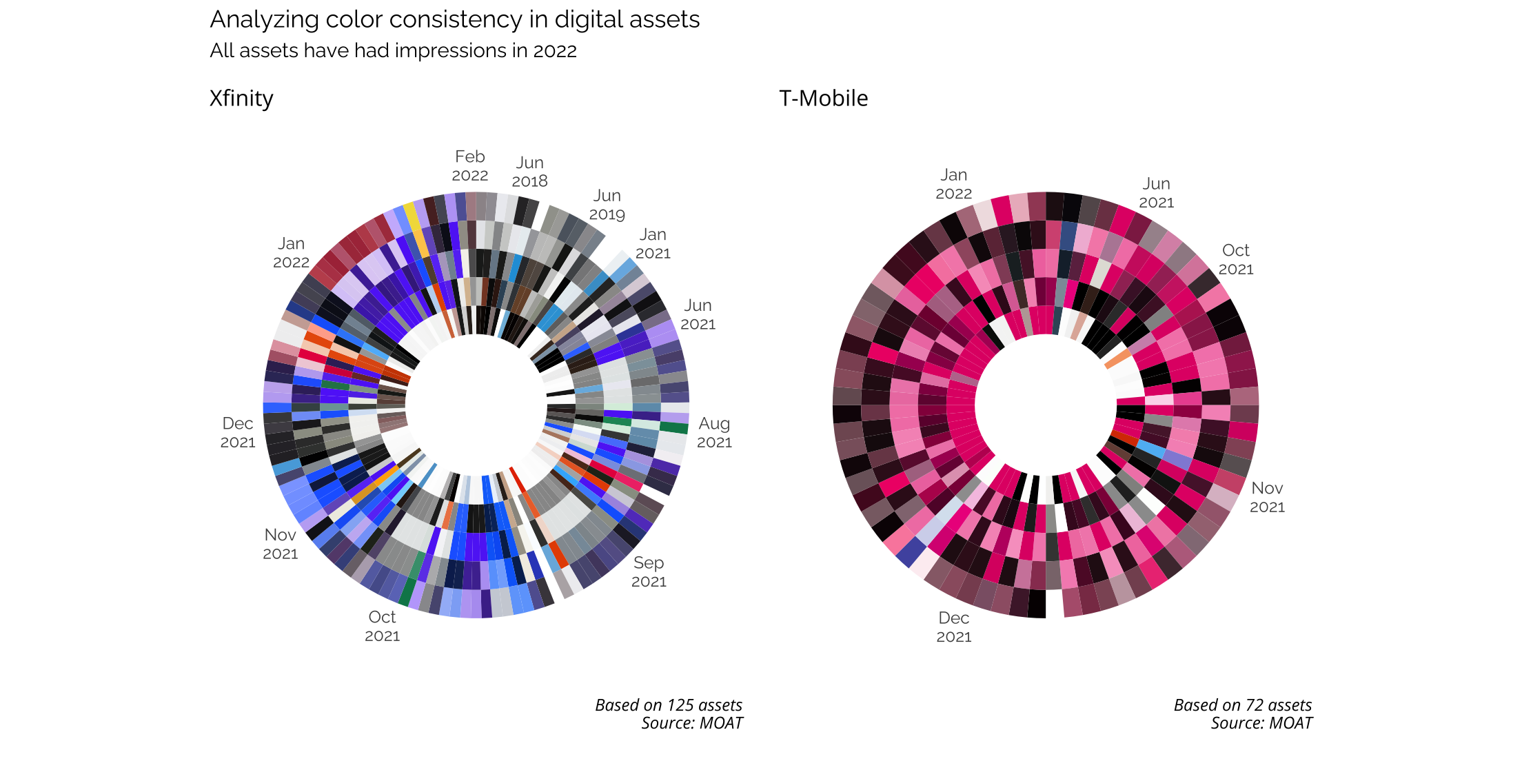
We’re only going to keep display assets that have been live in 2022, and since we’re going to plot these in a wheel, we’re going to arrange each asset by when it was first seen in-market. This way, our wheel can be read in a type of chronological order in terms of colors. This should allow for easy visual inspection as to the consistency of color usage.
# function to quantize colors from display assets
get_colorPal <- function(im, n, cs){
  image_read(im) %>%
    image_resize("500") %>%
    image_quantize(max=n, colorspace=cs) %>%  ## reducing colours! different colorspace gives you different result
    magick2cimg() %>%  ## I'm converting, becauase I want to use as.data.frame function in imager package.
    RGBtoHSV() %>% ## i like sorting colour by hue rather than RGB (red green blue)
    as.data.frame(wide="c") %>%  #3 making it wide makes it easier to output hex colour
    mutate(hex=hsv(rescale(c.1, from=c(0,360)),c.2,c.3),
           hue = c.1,
           sat = c.2,
           value = c.3) %>%
    count(hex, hue, sat,value, sort=T) %>%
    mutate(colorspace = cs) %>%
    select(colorspace,hex,hue,sat,value,n)

# keep assets seen in 2022 and pass through function
xfi <- xfi %>%
  mutate(first_year = lubridate::year(as.Date(first_seen)),
         last_year = lubridate::year(as.Date(last_seen)),
         floor_month = lubridate::floor_date(as.Date(first_seen), "month")) %>%
  filter(last_year == "2022") %>%
  arrange(first_seen) %>%
  mutate(n = 5, cs = "Lab") %>%
  mutate(colors = pmap(list(screenshot, n, cs), get_colorPal)) %>%
  nest(data = c(n, cs))
}
Plotting
With our data, we just need to identify each individual asset with a distinct id and then plot it using coord_polar() and we have a wheel that shows the colors of of digital display.
xfi %>%
  mutate(id = row_number()) %>%
  unnest(cols = colors) %>%
  group_by(id) %>%
  mutate(ypos=row_number(hue)) %>%  ## alter stacking order
  ggplot(aes(x=id, y=ypos, fill=hex)) +
  geom_tile() +
  scale_fill_identity() +
  scale_y_continuous(breaks=NULL) +
  theme_twg() +
  coord_polar() +
  expand_limits(y=-2)
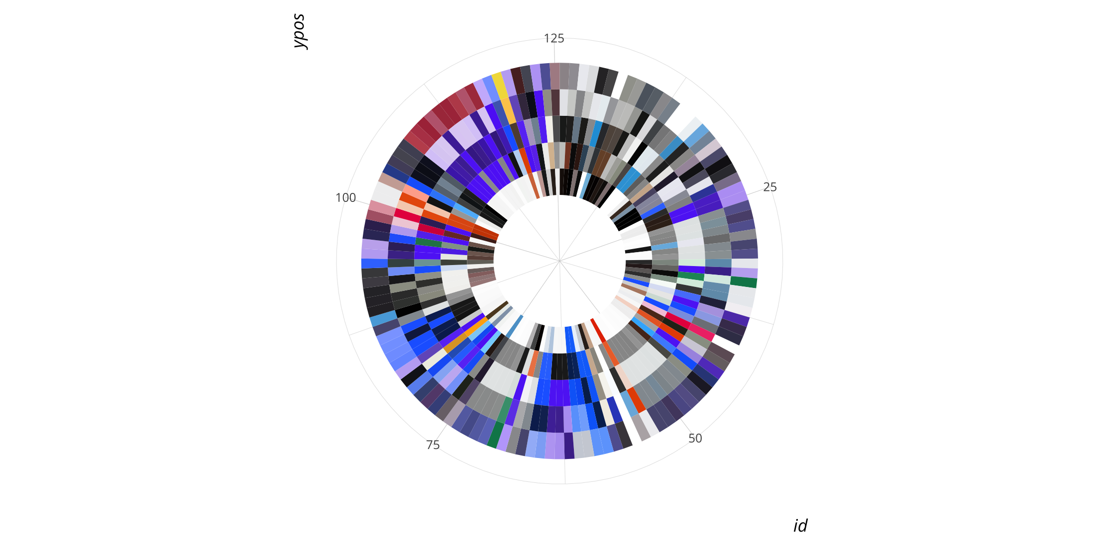
From the plot, we can see just how many different colors are being used, and since we’re in an ordered fashion, we can use the wheel to identify display assets with stranger color usage. For instance, we see green suddenly show up in plot 34, and when we call it, we find that it’s a regional ad that’s co-branded with the Philadelphia Eagles.
image_ggplot(image_read(xfi$screenshot[34]))

Comparing to another brand
As a point of comparison, let’s compare the Xfinity color wheel to that of T-Mobile’s 2022 digital assets.